If you've worked on advanced dynamics problems, you know deriving equations of motion by hand can be brutal. Most courses jump straight to matrices and numerical methods. Here I'll show how I use sympy.physics.mechanics to get symbolic equations of motion, then integrate them numerically for simulation.
Below is an interactive example — a basketball spinning on a finger. Orbit with your mouse and tweak initial conditions:
Why symbolic mechanics?
Pros
- Vectors can live in different frames; SymPy handles rotation matrices when you combine them.
- You get exact symbolic results, not just floating-point approximations.
- Helpers like
e_b.ang_vel_in(N)ande_b.dcm(N)skip tedious intermediate steps.
Cons
- Documentation and examples for
sympy.physics.mechanicsare sparse. - You should still learn the pencil-and-paper version in a dynamics course — it's how you catch nonsense answers.
Prerequisites
- Basic dynamics (Euler's laws, rotating frames)
- Comfortable with Python
Code: Jupyter notebook on GitHub · Three.js simulation source
Step 1 — Reference frames (3-1-3 Euler sequence)
from IPython.display import Markdown
import sympy as sp
from sympy.physics.mechanics import *

theta, phi, psi = dynamicsymbols('theta phi psi')

N = ReferenceFrame('N')
A = N.orientnew('A', 'Axis', [phi, N.z])
B = A.orientnew('B', 'Axis', [theta, A.x])
e_b = B.orientnew('e_b', 'Axis', [psi, B.z])

omega = e_b.ang_vel_in(N)
The dynamic symbols $\theta$, $\phi$, $\psi$ are functions of time. Frame A rotates about $N.z$ by $\phi$, B about $A.x$ by $\theta$, and e_b about $B.z$ by $\psi$.
Visualize the sequence (set dropdown to 313):
Angular velocity of $e_b$ in $N$:
omega = e_b.ang_vel_in(N)
omega.express(e_b)  # or omega.express(N)
Step 2 — Kinematics (rolling constraint)
t = sp.symbols('t')
r = sp.symbols('r')

P = Point('P')                          # contact point
CM = P.locatenew('CM', r * e_b.z)
r_P_CM = CM.pos_from(P)

P.set_vel(N, 0)
P.set_vel(e_b, 0)
CM.set_vel(e_b, 0)
CM.set_vel(N, omega.cross(r_P_CM))
- Contact point P is fixed in $N$ (still finger) and in $e_b$ (bottom of ball).
- CM has zero velocity in the body frame.
- Rolling: $\vec{v}_{CM/N} = \omega_{b/N} \times \vec{r}_{P \rightarrow CM}$.
Velocities and accelerations:
CM.vel(N).express(e_b)
CM.acc(N).express(e_b)
Step 3 — Kinetics (Euler's laws)
m, g, t = sp.symbols('m g t')

Ixx = 2 * m * r**2 / 5
Iyy = Ixx
Izz = Ixx
I_c = inertia(e_b, Ixx, Iyy, Izz)

Fg = -m * g * N.z
Fr = m * CM.acc(N) - Fg

Hc = I_c.dot(omega)
Hcdot = Hc.diff(t, N)
r_p = -r_P_CM
M = r_p.cross(Fr)

fancyWayToWriteZero = Hcdot - M
For a uniform sphere, $I = \frac{2}{5}mr^2$ about any body axis.
- First law: $\sum \vec{F} = m\vec{a}$ → reaction force $\vec{F}_r = m\vec{a}_{CM} - \vec{F}_g$.
- Second law: $\sum \vec{M} = \dot{\vec{H}}_c$ with $\vec{H}_c = I\omega$.
Step 4 — Solve symbolically
SymPy doesn't reduce vector equations directly, so project onto body axes:
eq1 = dot(fancyWayToWriteZero, e_b.x)
eq2 = dot(fancyWayToWriteZero, e_b.y)
eq3 = dot(fancyWayToWriteZero, e_b.z)

sol = sp.solve([eq1, eq2, eq3],
               [psi.diff(t, 2), theta.diff(t, 2), phi.diff(t, 2)],
               dict=True)
Access $\ddot\psi$, $\ddot\theta$, $\ddot\phi$ via sol[0][psi.diff(t,2)], etc.
Step 5 — Integrate and visualize
The hard part is done. Options:
| Approach | Integration | Visualization |
|---|---|---|
| Notebook | scipy.integrate.odeint |
Manim (FPS-limited) |
| Web demo | numeric Dormand–Prince |
Three.js |
Web rotation (camera-adjusted 2-3-2 sequence in Three.js):
let quaternion = new THREE.Quaternion();
quaternion.setFromEuler(new THREE.Euler(0, phi, 0, 'XYZ'));
quaternion.multiply(new THREE.Quaternion().setFromEuler(new THREE.Euler(0, 0, theta, 'XYZ')));
quaternion.multiply(new THREE.Quaternion().setFromEuler(new THREE.Euler(0, psi, 0, 'XYZ')));
basketballOffset.setRotationFromQuaternion(quaternion);
Loop: integrate → sample $\psi, \theta, \phi$ at time $t$ → apply rotations → render.
More simulations
Explore other systems I built with the same pipeline:
- Rolling coin — 3-1-2 sequence; stable spin at high $\dot\psi_0$
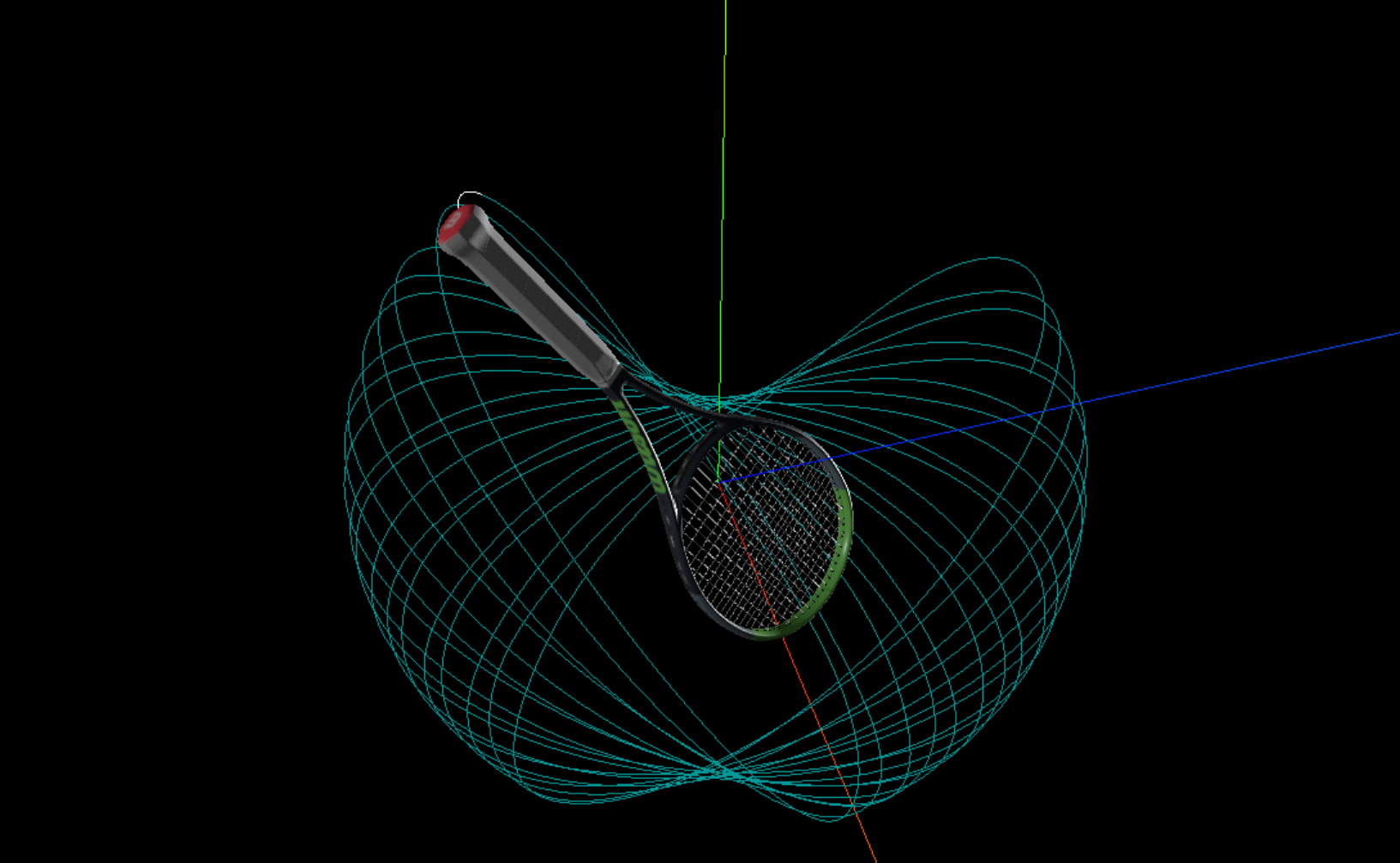
- Intermediate axis theorem — unstable spin about $I_2$
- Euler angle explorer
That's the workflow — symbolic setup in SymPy, numerical integration, then whatever renderer you like. Hope it helps.